A distribution geoms that fills the panel and works with discrete and continuous data

These versions of the histogram and density geoms have been designed specifically for diagonal plotting with facet_matrix(). They differ from ggplot2::geom_histogram() and ggplot2::geom_density() in that they defaults to mapping x and y to .panel_x and .panel_y respectively, they ignore the y scale of the panel and fills it out, and they work for both continuous and discrete x scales.

geom_autodensity(
  mapping = NULL,
  data = NULL,
  stat = "autodensity",
  position = "floatstack",
  ...,
  bw = "nrd0",
  adjust = 1,
  kernel = "gaussian",
  n = 512,
  trim = FALSE,
  na.rm = FALSE,
  show.legend = NA,
  inherit.aes = TRUE,
  outline.type = "upper"
)

geom_autohistogram(
  mapping = NULL,
  data = NULL,
  stat = "autobin",
  position = "floatstack",
  ...,
  bins = NULL,
  na.rm = FALSE,
  show.legend = NA,
  inherit.aes = TRUE
)

Arguments

mapping

Set of aesthetic mappings created by aes(). If specified and inherit.aes = TRUE (the default), it is combined with the default mapping at the top level of the plot. You must supply mapping if there is no plot mapping.

data

The data to be displayed in this layer. There are three options:

If NULL, the default, the data is inherited from the plot data as specified in the call to ggplot().

A data.frame, or other object, will override the plot data. All objects will be fortified to produce a data frame. See fortify() for which variables will be created.

A function will be called with a single argument, the plot data. The return value must be a data.frame, and will be used as the layer data. A function can be created from a formula (e.g. ~ head(.x, 10)).

stat

The statistical transformation to use on the data for this layer, either as a ggproto Geom subclass or as a string naming the stat stripped of the stat_ prefix (e.g. "count" rather than "stat_count")

position

Position adjustment, either as a string naming the adjustment (e.g. "jitter" to use position_jitter), or the result of a call to a position adjustment function. Use the latter if you need to change the settings of the adjustment.

...

Other arguments passed on to layer(). These are often aesthetics, used to set an aesthetic to a fixed value, like colour = "red" or size = 3. They may also be parameters to the paired geom/stat.

bw

The smoothing bandwidth to be used. If numeric, the standard deviation of the smoothing kernel. If character, a rule to choose the bandwidth, as listed in stats::bw.nrd(). Note that automatic calculation of the bandwidth does not take weights into account.

adjust

A multiplicate bandwidth adjustment. This makes it possible to adjust the bandwidth while still using the a bandwidth estimator. For example, adjust = 1/2 means use half of the default bandwidth.

kernel

Kernel. See list of available kernels in density().

n

number of equally spaced points at which the density is to be estimated, should be a power of two, see density() for details

trim

If FALSE, the default, each density is computed on the full range of the data. If TRUE, each density is computed over the range of that group: this typically means the estimated x values will not line-up, and hence you won't be able to stack density values. This parameter only matters if you are displaying multiple densities in one plot or if you are manually adjusting the scale limits.

na.rm

If FALSE, the default, missing values are removed with a warning. If TRUE, missing values are silently removed.

show.legend

logical. Should this layer be included in the legends? NA, the default, includes if any aesthetics are mapped. FALSE never includes, and TRUE always includes. It can also be a named logical vector to finely select the aesthetics to display.

inherit.aes

If FALSE, overrides the default aesthetics, rather than combining with them. This is most useful for helper functions that define both data and aesthetics and shouldn't inherit behaviour from the default plot specification, e.g. borders().

outline.type

Type of the outline of the area; "both" draws both the upper and lower lines, "upper"/"lower" draws the respective lines only. "full" draws a closed polygon around the area.

bins

Number of bins. Overridden by binwidth. Defaults to 30.

Examples

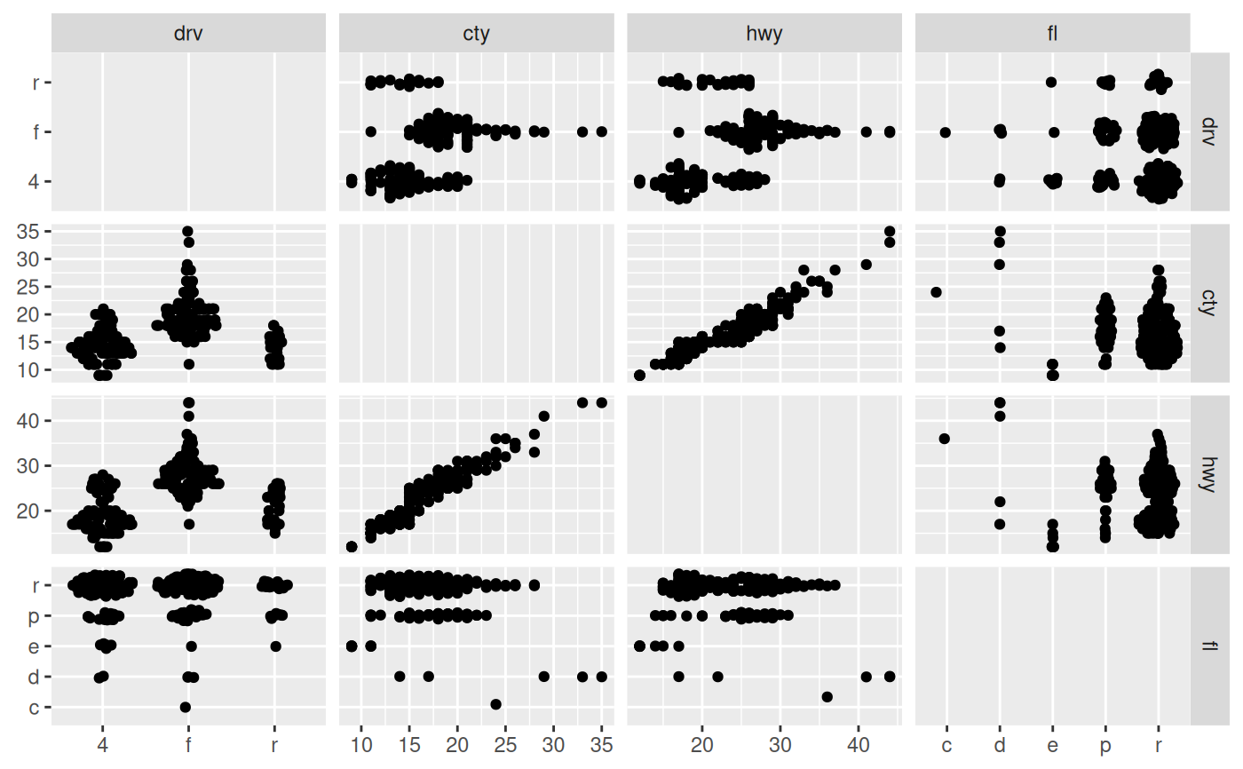
# A matrix plot with a mix of discrete and continuous variables
p <- ggplot(mpg) +
  geom_autopoint() +
  facet_matrix(vars(drv:fl), layer.diag = 2, grid.y.diag = FALSE)
p


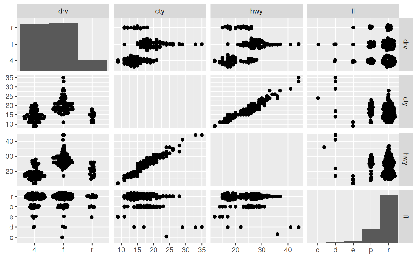
# Diagonal histograms
p + geom_autohistogram()


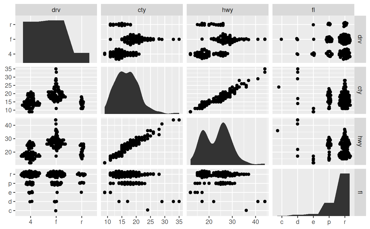
# Diagonal density distributions
p + geom_autodensity()


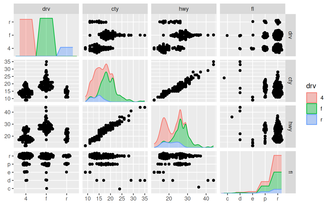
# You can use them like regular layers with groupings etc
p + geom_autodensity(aes(colour = drv, fill = drv),
                     alpha = 0.4)

A distribution geoms that fills the panel and works with discrete and continuous data

Arguments

See also

Examples