This geom lets you annotate sets of points via rectangles. The rectangles are
simply scaled to the range of the data and as with the other
geom_mark_*() geoms expanded and have rounded corners.
Usage
geom_mark_rect(
  mapping = NULL,
  data = NULL,
  stat = "identity",
  position = "identity",
  expand = unit(5, "mm"),
  radius = unit(2.5, "mm"),
  label.margin = margin(2, 2, 2, 2, "mm"),
  label.width = NULL,
  label.minwidth = unit(50, "mm"),
  label.hjust = 0,
  label.fontsize = 12,
  label.family = "",
  label.lineheight = 1,
  label.fontface = c("bold", "plain"),
  label.fill = "white",
  label.colour = "black",
  label.buffer = unit(10, "mm"),
  con.colour = "black",
  con.size = 0.5,
  con.type = "elbow",
  con.linetype = 1,
  con.border = "one",
  con.cap = unit(3, "mm"),
  con.arrow = NULL,
  ...,
  na.rm = FALSE,
  show.legend = NA,
  inherit.aes = TRUE
)
Arguments
- mapping
Set of aesthetic mappings created by
aes(). If specified andinherit.aes = TRUE(the default), it is combined with the default mapping at the top level of the plot. You must supplymappingif there is no plot mapping.- data
The data to be displayed in this layer. There are three options:
If
NULL, the default, the data is inherited from the plot data as specified in the call toggplot().A
data.frame, or other object, will override the plot data. All objects will be fortified to produce a data frame. Seefortify()for which variables will be created.A
functionwill be called with a single argument, the plot data. The return value must be adata.frame, and will be used as the layer data. Afunctioncan be created from aformula(e.g.~ head(.x, 10)).- stat
The statistical transformation to use on the data for this layer. When using a
geom_*()function to construct a layer, thestatargument can be used the override the default coupling between geoms and stats. Thestatargument accepts the following:A
Statggproto subclass, for exampleStatCount.A string naming the stat. To give the stat as a string, strip the function name of the
stat_prefix. For example, to usestat_count(), give the stat as"count".For more information and other ways to specify the stat, see the layer stat documentation.
- position
A position adjustment to use on the data for this layer. This can be used in various ways, including to prevent overplotting and improving the display. The
positionargument accepts the following:The result of calling a position function, such as
position_jitter(). This method allows for passing extra arguments to the position.A string naming the position adjustment. To give the position as a string, strip the function name of the
position_prefix. For example, to useposition_jitter(), give the position as"jitter".For more information and other ways to specify the position, see the layer position documentation.
- expand
A numeric or unit vector of length one, specifying the expansion amount. Negative values will result in contraction instead. If the value is given as a numeric it will be understood as a proportion of the plot area width.
- radius
As
expandbut specifying the corner radius.- label.margin
The margin around the annotation boxes, given by a call to
ggplot2::margin().- label.width
A fixed width for the label. Set to
NULLto let the text orlabel.minwidthdecide.- label.minwidth
The minimum width to provide for the description. If the size of the label exceeds this, the description is allowed to fill as much as the label.
- label.hjust
The horizontal justification for the annotation. If it contains two elements the first will be used for the label and the second for the description.
- label.fontsize
The size of the text for the annotation. If it contains two elements the first will be used for the label and the second for the description.
- label.family
The font family used for the annotation. If it contains two elements the first will be used for the label and the second for the description.
- label.lineheight
The height of a line as a multipler of the fontsize. If it contains two elements the first will be used for the label and the second for the description.
- label.fontface
The font face used for the annotation. If it contains two elements the first will be used for the label and the second for the description.
- label.fill
The fill colour for the annotation box. Use
"inherit"to use the fill from the enclosure or"inherit_col"to use the border colour of the enclosure.- label.colour
The text colour for the annotation. If it contains two elements the first will be used for the label and the second for the description. Use
"inherit"to use the border colour of the enclosure or"inherit_fill"to use the fill colour from the enclosure.- label.buffer
The size of the region around the mark where labels cannot be placed.
- con.colour
The colour for the line connecting the annotation to the mark. Use
"inherit"to use the border colour of the enclosure or"inherit_fill"to use the fill colour from the enclosure.- con.size
The width of the connector. Use
"inherit"to use the border width of the enclosure.- con.type
The type of the connector. Either
"elbow","straight", or"none".- con.linetype
The linetype of the connector. Use
"inherit"to use the border linetype of the enclosure.- con.border
The bordertype of the connector. Either
"one"(to draw a line on the horizontal side closest to the mark),"all"(to draw a border on all sides), or"none"(not going to explain that one).- con.cap
The distance before the mark that the line should stop at.
- con.arrow
An arrow specification for the connection using
grid::arrow()for the end pointing towards the mark.- ...
Other arguments passed on to
layer()'sparamsargument. These arguments broadly fall into one of 4 categories below. Notably, further arguments to thepositionargument, or aesthetics that are required can not be passed through.... Unknown arguments that are not part of the 4 categories below are ignored.Static aesthetics that are not mapped to a scale, but are at a fixed value and apply to the layer as a whole. For example,
colour = "red"orlinewidth = 3. The geom's documentation has an Aesthetics section that lists the available options. The 'required' aesthetics cannot be passed on to theparams. Please note that while passing unmapped aesthetics as vectors is technically possible, the order and required length is not guaranteed to be parallel to the input data.When constructing a layer using a
stat_*()function, the...argument can be used to pass on parameters to thegeompart of the layer. An example of this isstat_density(geom = "area", outline.type = "both"). The geom's documentation lists which parameters it can accept.Inversely, when constructing a layer using a
geom_*()function, the...argument can be used to pass on parameters to thestatpart of the layer. An example of this isgeom_area(stat = "density", adjust = 0.5). The stat's documentation lists which parameters it can accept.The
key_glyphargument oflayer()may also be passed on through.... This can be one of the functions described as key glyphs, to change the display of the layer in the legend.
- na.rm
If
FALSE, the default, missing values are removed with a warning. IfTRUE, missing values are silently removed.- show.legend
logical. Should this layer be included in the legends?
NA, the default, includes if any aesthetics are mapped.FALSEnever includes, andTRUEalways includes. It can also be a named logical vector to finely select the aesthetics to display.- inherit.aes
If
FALSE, overrides the default aesthetics, rather than combining with them. This is most useful for helper functions that define both data and aesthetics and shouldn't inherit behaviour from the default plot specification, e.g.borders().
Aesthetics
geom_mark_rect understands the following aesthetics (required aesthetics are
in bold):
x
y
x0 (used to anchor the label)
y0 (used to anchor the label)
filter
label
description
color
fill
group
size
linetype
alpha
Annotation
All geom_mark_* allow you to put descriptive textboxes connected to the
mark on the plot, using the label and description aesthetics. The
textboxes are automatically placed close to the mark, but without obscuring
any of the datapoints in the layer. The placement is dynamic so if you resize
the plot you'll see that the annotation might move around as areas become big
enough or too small to fit the annotation. If there's not enough space for
the annotation without overlapping data it will not get drawn. In these cases
try resizing the plot, change the size of the annotation, or decrease the
buffer region around the marks.
Filtering
Often marks are used to draw attention to, or annotate specific features of
the plot and it is thus not desirable to have marks around everything. While
it is possible to simply pre-filter the data used for the mark layer, the
geom_mark_* geoms also comes with a dedicated filter aesthetic that, if
set, will remove all rows where it evalutates to FALSE. There are
multiple benefits of using this instead of prefiltering. First, you don't
have to change your data source, making your code more adaptable for
exploration. Second, the data removed by the filter aesthetic is remembered
by the geom, and any annotation will take care not to overlap with the
removed data.
See also
Other mark geoms:
geom_mark_circle(),
geom_mark_ellipse(),
geom_mark_hull()
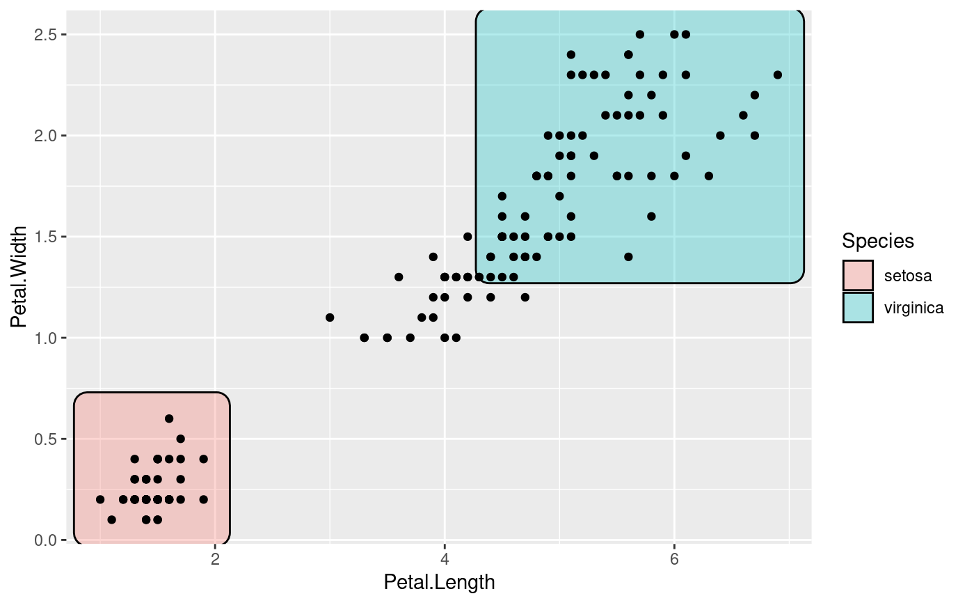
Examples
ggplot(iris, aes(Petal.Length, Petal.Width)) +
geom_mark_rect(aes(fill = Species, filter = Species != 'versicolor')) +
geom_point()
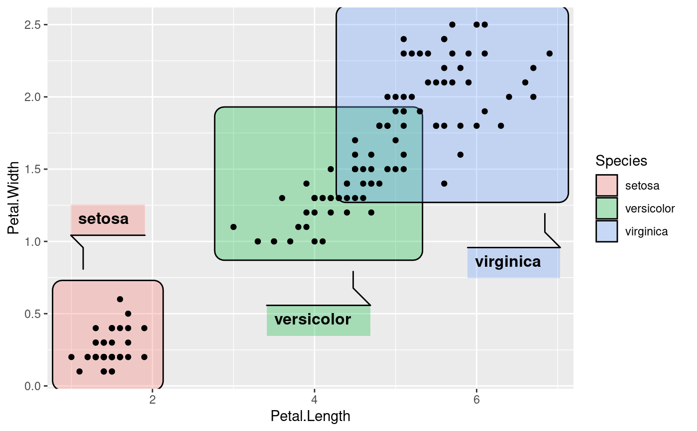
 # Add annotation
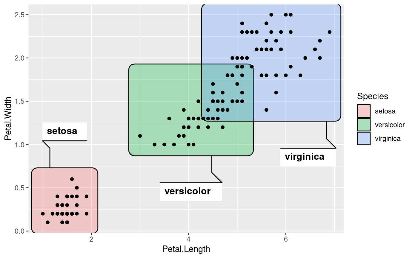
ggplot(iris, aes(Petal.Length, Petal.Width)) +
geom_mark_rect(aes(fill = Species, label = Species)) +
geom_point()
# Add annotation
ggplot(iris, aes(Petal.Length, Petal.Width)) +
geom_mark_rect(aes(fill = Species, label = Species)) +
geom_point()
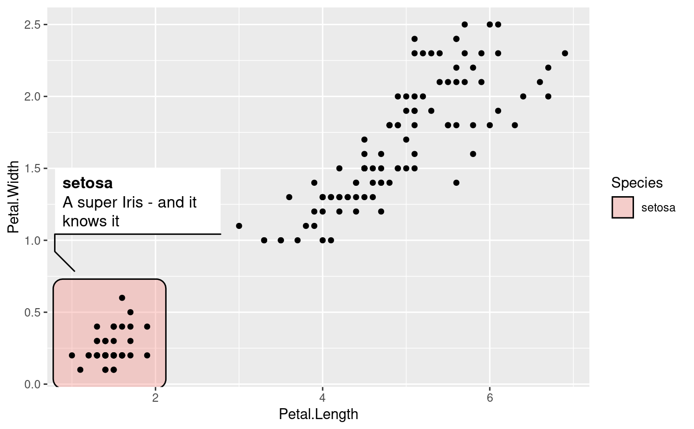
 # Long descriptions are automatically wrapped to fit into the width
iris$desc <- c(
'A super Iris - and it knows it',
'Pretty mediocre Iris, but give it a couple of years and it might surprise you',
"You'll never guess what this Iris does every Sunday"
)[iris$Species]
ggplot(iris, aes(Petal.Length, Petal.Width)) +
geom_mark_rect(aes(fill = Species, label = Species, description = desc,
filter = Species == 'setosa')) +
geom_point()
# Long descriptions are automatically wrapped to fit into the width
iris$desc <- c(
'A super Iris - and it knows it',
'Pretty mediocre Iris, but give it a couple of years and it might surprise you',
"You'll never guess what this Iris does every Sunday"
)[iris$Species]
ggplot(iris, aes(Petal.Length, Petal.Width)) +
geom_mark_rect(aes(fill = Species, label = Species, description = desc,
filter = Species == 'setosa')) +
geom_point()
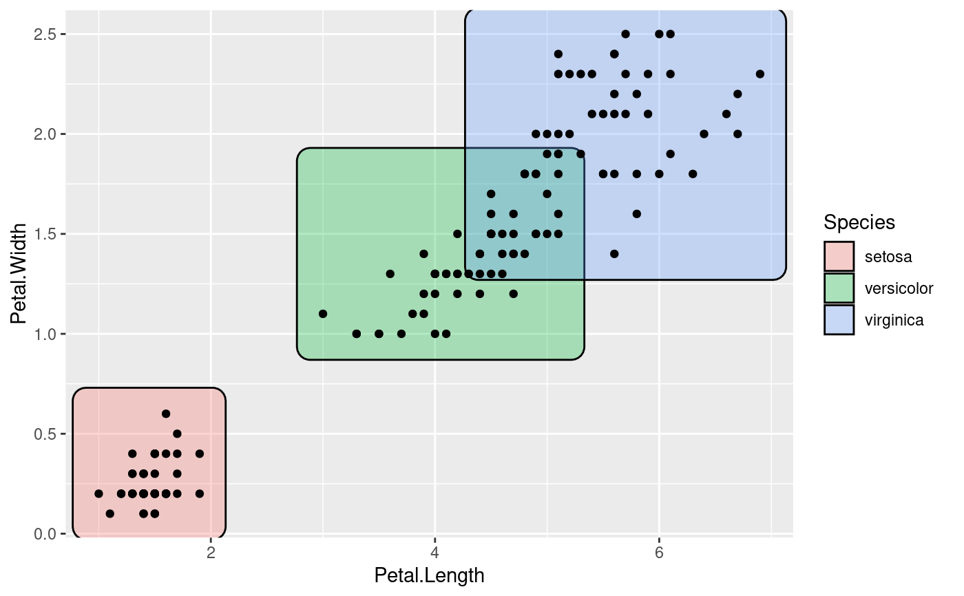
 # Change the buffer size to move labels farther away (or closer) from the
# marks
ggplot(iris, aes(Petal.Length, Petal.Width)) +
geom_mark_rect(aes(fill = Species, label = Species),
label.buffer = unit(30, 'mm')) +
geom_point()
# Change the buffer size to move labels farther away (or closer) from the
# marks
ggplot(iris, aes(Petal.Length, Petal.Width)) +
geom_mark_rect(aes(fill = Species, label = Species),
label.buffer = unit(30, 'mm')) +
geom_point()
 # The connector is capped a bit before it reaches the mark, but this can be
# controlled
ggplot(iris, aes(Petal.Length, Petal.Width)) +
geom_mark_rect(aes(fill = Species, label = Species),
con.cap = 0) +
geom_point()
# The connector is capped a bit before it reaches the mark, but this can be
# controlled
ggplot(iris, aes(Petal.Length, Petal.Width)) +
geom_mark_rect(aes(fill = Species, label = Species),
con.cap = 0) +
geom_point()
 # If you want to use the scaled colours for the labels or connectors you can
# use the "inherit" keyword instead
ggplot(iris, aes(Petal.Length, Petal.Width)) +
geom_mark_rect(aes(fill = Species, label = Species),
label.fill = "inherit") +
geom_point()
# If you want to use the scaled colours for the labels or connectors you can
# use the "inherit" keyword instead
ggplot(iris, aes(Petal.Length, Petal.Width)) +
geom_mark_rect(aes(fill = Species, label = Species),
label.fill = "inherit") +
geom_point()